
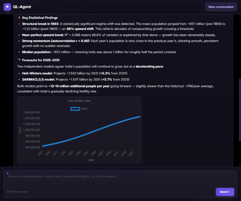
Our first two articles on QuantumLayers covered the platform from the outside in: the databases and APIs it connects to, how it merges sources, the summary statistics, correlations and ANOVA tests it runs, and the reports and monitors that deliver results. One feature got only a paragraph each time, and it's arguably the most ambitious part of the product: the insight engine.
When you ask QuantumLayers to generate insights for a dataset, it doesn't run one analysis. It runs a battery of them, from distribution checks and correlations to regression models, time-series diagnostics and forecasts. Then it scores every finding and returns a ranked list, with a plain-language message, a recommendation and a suggested chart for each.
To see what that looks like in practice, we pointed it at three public datasets that QuantumLayers pulls in through its API connector: 35 years of monthly climate records from NOAA's Central Park weather station in New York, ten years of daily weather for Berlin from Open-Meteo, and the International Monetary Fund's real GDP growth figures for eight major economies from 1980 onward. Public data makes a good test because the real-world history is known. If the engine claims something happened, we can check whether it did.
What follows is a tour of the kinds of findings the engine produces, what each one means, how it's computed, and when to trust it. Some results are impressive. A few are good examples of why automated findings still need a human reader.
How a finding is structured
Every insight QuantumLayers returns has the same anatomy, and knowing it makes the output much easier to work with.
Each finding has a type, such as forecast, structural break, correlation, outliers or predictive model. It has a severity label (positive, info, warning, medium or high) that says whether it's good news, neutral information or something that needs attention. It has an importance score, which the engine uses to rank findings so the most consequential ones come first. The plain-language message says what was found, and the recommendation says what to do about it. Most findings also include a suggested chart, such as a time series for a trend, a scatter plot for a relationship or a box plot for outliers, ready to save or share.
Underneath the prose, each finding carries metadata: the test statistic, the threshold it was compared against, model parameters, forecast values and error measures. This is what makes the engine auditable. You never have to take a sentence like "a structural break was detected" on faith, because the CUSUM statistic and the critical value it beat are right there.
When the engine tests many things at once, it also controls for false discoveries. Findings that rely on a significance test carry an adjusted p-value and a flag showing whether they survive a false discovery rate (FDR) correction. This matters more than it sounds. Running dozens of tests on one dataset guarantees that a few will look significant by pure chance, and FDR correction is the standard way to keep that from flooding your results with noise.
Time series: what the engine looks for
As soon as a dataset has a date column, the engine switches on a set of time-series analyses. It aggregates the data to a sensible interval (daily records into weeks, monthly records into years, and so on) and then looks at the series from several angles.
Structural breaks: when the rules change
A structural break is a point where a series shifts to a new level and stays there. Think of a pricing change that permanently lifts average order value, a competitor's launch that lowers your baseline signups, or a change in how a metric is measured. Breaks matter because they invalidate simple trend lines. A straight line drawn through data that changed regime halfway through describes neither period.
QuantumLayers detects breaks with a CUSUM test. CUSUM stands for cumulative sum, and the idea is intuitive. Walk through the series adding up how far each value sits from the overall average. If the series is stable, those deviations cancel out and the running total wanders around zero. If the series shifted partway through, the running total drifts steadily one way before the break and back the other way after it. The test statistic measures how far that drift goes, and the engine flags a break when it exceeds the 5% critical value of 1.36. It reports the break date, the mean before and after, and the percentage change.
The IMF data provided a perfect check. The engine found a break in Japan's GDP growth around 1991, with average annual growth falling from 4.3% before to 0.8% after. That's the bursting of Japan's asset-price bubble and the start of what became known as its lost decades. It also found a break in China's growth around 2011, with the average dropping from 10.1% to 5.4%. That matches the well-documented end of China's double-digit expansion. The engine knew nothing about economic history. It found both turning points from the numbers alone, and the CUSUM statistics (2.05 for Japan, 2.41 for China) cleared the threshold comfortably.
The climate data produced a subtler result. At Central Park, the engine found an upward break in the average monthly minimum temperature around 2009, with the mean rising from 8.86°C to 9.72°C. The average temperature showed a smaller break at the same point. This is consistent with warming nights, but it's also the kind of finding that deserves a second question, because a break can also come from a change in instruments, station siting or data processing.
The Berlin data shows why that second question matters. The engine found a 14% upward break in maximum daily wind speed in February 2017. That may be real, but wind data from weather models is known to shift when the underlying model or its inputs change. A structural break tells you something changed. It doesn't tell you whether the world changed or the measurement did. In business data, the same caution applies: a sudden lift in conversions might be a successful campaign, or it might be a tracking script that started double-counting.
Lead and lag: finding leading indicators
Some of the most valuable business insights are leading indicators: a metric that moves before another one does. Trial signups that predict paid conversions two months later. Support tickets that rise ahead of churn. Pipeline value that foreshadows next quarter's revenue.
QuantumLayers looks for these with cross-correlation analysis. It shifts one series forward and backward in time against another and measures the correlation at each offset, or lag. If the correlation peaks at a nonzero lag and clears a significance threshold, the engine reports which series leads, by how much and how strongly.
An important technical detail: the engine runs this analysis on first-differenced data, meaning the change from one period to the next rather than the raw level. That's the right call. Two series that both trend upward over time, such as your revenue and the global population, will show a strong correlation at every lag simply because they both go up. Differencing removes the shared trend and asks a better question: when one series moves more than usual, does the other follow?
The climate data also shows the limits of this analysis. Aggregated to annual values, the engine reported that the average temperature at Central Park "leads" the maximum temperature by four years, with a cross-correlation of 0.39 against a threshold of 0.34. That's statistically above the bar, but physically it makes no sense. The average temperature is essentially the midpoint of the daily highs and lows, so it can't anticipate the highs by four years. The problem is the sample: 35 annual values, tested at many different lags. With that little data and that many comparisons, one lag will usually clear the threshold by chance.
The lesson generalizes. Treat a lead-lag finding as a hypothesis, not a conclusion, especially when the correlation barely clears the threshold and the series is short. A leading indicator worth acting on should make business sense, show up at a plausible lag and hold up when you check it again on new data. That last check is something a QuantumLayers monitor can do for you, as we'll see.
Autocorrelation: does the series remember?
Autocorrelation measures how strongly a series is related to its own past. Positive autocorrelation means momentum: good months tend to follow good months. Negative autocorrelation means alternation: a high value tends to be followed by a low one, a pattern typical of mean reversion or of over-correction, such as inventory orders that overshoot and then undershoot.
For Central Park's annual precipitation, the engine found strong negative autocorrelation in the year-to-year changes (r = −0.53). In plain terms, an unusually wet year tends to be followed by a drier one. Some of that is natural variability. Some of it is a known mathematical effect: when a series is mostly random noise, the year-to-year differences are negatively correlated almost automatically, because a spike up is followed by a drop back to normal. It's a useful finding to know about, mostly as a warning against reading too much into a single wet or dry year.
Forecasting: Holt-Winters and SARIMA
When a dataset has at least 12 periods of history, the engine produces forecasts using two established families of models, and it reports enough detail to judge them.
Holt-Winters is exponential smoothing in up to three layers. Single smoothing tracks the level of a series, giving recent observations more weight than old ones. Double smoothing adds a trend. Triple smoothing adds seasonality, such as the regular rise and fall of retail sales through the year. QuantumLayers reports which variant it used and its smoothing parameters. Alpha controls how quickly the level reacts to new data, beta how quickly the trend adapts, and gamma how quickly the seasonal pattern updates. Each runs from 0 to 1, and higher values mean the model reacts faster and forgets the past sooner. It also reports the RMSE (root mean squared error), the typical size of the model's errors in the units of the data.
SARIMA (seasonal autoregressive integrated moving average) takes a different approach. It models each value as a combination of past values and past forecast errors, after differencing the series to remove trends. The engine reports the model's order in the standard notation. A SARIMA(2,1,1) uses two past values (the autoregressive part), differences the data once to remove a trend (the integrated part), and uses one past error term (the moving-average part). Our IMF results used both (2,1,1) and (2,0,1) models, depending on whether a series needed differencing.
The two methods have different strengths. Holt-Winters is robust and easy to interpret, and it works well for business series with steady trends and seasons. SARIMA can capture more complex dynamics but needs more data and is more sensitive to how it's specified. When the engine produces both for related series, its recommendations sometimes suggest cross-checking one against the other. When they agree, you can be more confident. When they disagree, the future is genuinely uncertain.
How to read a forecast without being misled
Our tests surfaced three reading rules that will save you from the most common forecasting mistakes.
First, look at the levels, not just the percentage. For Germany, the engine projected GDP growth to "increase by 148.5%," and for Japan to "decrease by 101.1%." Those numbers are arithmetically correct and practically misleading. German growth was forecast to rise from about 0.6% to about 1.5% a year, and Japanese growth to drift from about 0.6% to roughly zero. When the starting value is close to zero, percentage changes explode. With growth rates, interest rates, margins or any other figure that is already a percentage, read the forecast values in the metadata and think in percentage points.
The Berlin forecast shows a related trap. The engine projected weekly maximum temperatures to rise 121% over 12 weeks, from about 2.7°C to 5.9°C. That's a sensible seasonal forecast, because the data ends in winter and spring is coming. But Celsius has an arbitrary zero, so "121% warmer" has no physical meaning. The forecast values are useful; the percentage isn't.
Second, check the error. The Holt-Winters forecast for Berlin's weekly temperatures carried an RMSE of 3.8°C, about the same size as the forecast change itself. The China forecast had an RMSE of 2.8 percentage points on a series that was projected to fall from 3.3% to 1.8%. When the typical error is as large as the change being forecast, treat the direction as a tendency and the specific values as rough guides.
Third, know what's already in your data. The IMF dataset runs to 2031, because the IMF publishes its own projections several years ahead. QuantumLayers treats those years as history, so its forecasts extend the IMF's projections rather than its actual figures. That's a forecast built on a forecast. In business data the equivalent is a budget column, a sales target or a pipeline estimate sitting in the same table as actual results. Before trusting any forecast, make sure the history it learned from really is history.
Predictive models and the multicollinearity check
Beyond time series, the engine also tries to explain each numeric column using the others. It fits a regression model and, when the model is strong, reports it as a finding: how much of the variation it explains (R²), how many predictors are significant, and which ones they are.
At Central Park, the engine's top-ranked finding was a model that predicts the maximum temperature with an R² of 1.000, a perfect fit, using the average and minimum temperatures. A perfect model sounds like a triumph. It isn't. As noted above, the average temperature is essentially the midpoint of the highs and lows. If you know the average and the minimum, you can calculate the maximum exactly. The model didn't discover anything; it rediscovered a definition.
Fortunately, the engine flagged this itself. Its second-ranked finding was a multicollinearity warning based on the variance inflation factor (VIF). VIF measures how much of one predictor can be explained by the others. A VIF of 1 means a predictor is independent of the rest, and the usual warning level is 5 or 10. The average temperature scored a VIF of about 58,000, meaning it was entirely determined by the other columns. Precipitation, which really is independent of temperature, scored 1.08. The engine's recommendation was to remove or combine the redundant variables.
This pairing is a good example of how to read the engine's output as a whole rather than one finding at a time. A very high R² next to very high VIF scores usually means the data contains derived columns: totals alongside their parts, a ratio alongside its numerator and denominator, or an average alongside the values it averages. In business datasets this is common. Revenue, units and price will always "predict" each other perfectly. The fix is to select only the columns that represent genuinely separate measurements before you generate insights, which QuantumLayers lets you do directly.
Distribution findings: outliers and skew
The engine also checks each numeric column's shape. For Berlin's daily rainfall, it reported a skewness of 9.5 and flagged 11.1% of the values (407 days) as outliers. It recommended a log transformation or the median instead of the mean.
Both findings are correct, and they're a good reminder that "outlier" doesn't mean "error." Rainfall is naturally lopsided. Most days are dry or nearly dry, and a minority of storms produce most of the total. Those 407 days aren't bad data; they're the rain. Revenue per customer, deal size, order value and incident duration behave the same way. The engine's job is to tell you the distribution is skewed so you summarize it correctly. Deciding whether an extreme value is a mistake or the most important event in the dataset is a judgment call the engine leaves to you.
The obvious findings and what they teach
Not every finding is interesting. For Berlin, four findings reported that weekly temperature and precipitation have a "statistically significant positive mean." The IMF data produced similar findings that India's and the United States' growth rates are consistently above zero. These are technically true and close to useless: rain can't be negative, and Berlin's weekly temperatures added up over seven days are above freezing most of the year.
These findings come from tests that ask whether a series is consistently above or below zero. In some data that's a valuable question. For a profit margin, a net promoter score, a cash flow or a forecast error, whether the average sits above zero is exactly what you want to know. For quantities that can only be positive, it's a formality.
The engine's ranking usually pushes such findings below more interesting ones, but not always. Two features help here. You can narrow the analysis to the columns you care about, and you can add a focus prompt, such as "focus on structural changes" or "look for leading indicators of churn," to steer the engine and its written narrative toward the questions that matter to you.
Public data as context for your own
All three datasets in this article came into QuantumLayers through its REST API connector, which handles the response format of many public sources directly: NOAA's climate records, Open-Meteo's weather service, the IMF's World Economic Outlook, and others such as the World Bank, FRED and the US Energy Information Administration. Once connected, a public dataset behaves like any other. It can be synced to pick up new releases, merged with your own data and analyzed.
That's where public data earns its place in a business analytics tool. A retailer can merge daily sales with local weather and see whether rain suppresses foot traffic. An exporter can line up its order volumes with GDP growth in its main markets and check whether demand follows the economic cycle. A solar installer can set its lead volume against irradiance data. Without that context, a sales dip in a wet month or a slow quarter in a slowing economy looks like a problem with your business. With it, you can separate what you control from what you don't.
The structural-break and lead-lag analyses are especially useful on merged data. If your sales show a break at the same point as a regional economic slowdown, that's informative. If a public indicator turns out to lead your demand by a quarter, you have an early-warning signal that someone else updates for free. Just remember the caution from earlier: confirm it makes sense and holds up over time before you plan around it.
Watching findings over time with monitors
Everything above describes a single run of the insight engine. Its real power shows when it runs repeatedly. A QuantumLayers monitor re-runs the engine on a schedule (hourly, daily, weekly or monthly) and compares the new findings with the previous ones. When a finding appears or disappears, it sends an alert.
For the finding types in this article, that's a natural fit. A new structural break in a key metric is exactly the kind of event you want to hear about the week it happens, not at the next quarterly review. A lead-lag relationship that keeps reappearing run after run is far more credible than one that showed up once, and a monitor gives you that history automatically. A forecast that shifts from an upward outlook to a downward one is worth an alert.
Monitors can be narrowed to specific columns, filtered to one segment or a date range, and capped at a number of tracked findings. Alerts go out by email, to a Slack channel, or as signed webhook events to another system. Webhook delivery can be limited to particular finding types, so a team can route structural breaks and forecast reversals to an operations channel while leaving routine distribution changes out. A cooldown setting stops a borderline finding from firing repeatedly as it crosses its threshold back and forth.
What this means for teams without a data team
Taken together, our tests give a clear picture of what the insight engine is good at and where it needs you.
It's good at breadth. In seconds, it runs analyses that would take an analyst days to set up: CUSUM break tests, cross-correlations on differenced data, regression with collinearity checks, Holt-Winters and SARIMA forecasts, outlier detection and false-discovery correction. It found the turning points in the Japanese and Chinese economies with no knowledge of either. It caught its own perfect-but-meaningless model with a VIF warning. And it exposes the statistics behind every sentence, so its claims can be checked.
It needs you for meaning. Statistics can't tell a measurement change from a real one, a definition from a discovery, or a lucky lag from a leading indicator. Percentage changes on rates and temperatures need translating back into levels. Forecasts built on projections need recognizing for what they are.
The practical approach is to read the ranked findings as a set of well-supported questions rather than a list of answers. Start with the top few, check the metadata behind any that would change a decision, ask whether each one makes sense for your business, and set a monitor to see which ones hold up as new data arrives. Used that way, the engine does the work of a junior analyst who never gets tired, and you do the part only someone who knows the business can.
Learn more and try it at quantumlayers.com.